Plots the objective function against two design variables
This function plots points at which the objective function was evaluated. The objective function points may be plotted in colour or black and white. The points may also be joined to represent the sequence of function evaluations.
Syntax
optimisationTrace(STRUCTOUT,STRUCTIN)
optimisationTrace(STRUCTOUT,STRUCTIN,PLOTTYPE)
optimisationTrace(STRUCTOUT,STRUCTIN,PLOTTYPE,FIG)
optimisationTrace(STRUCTOUT,STRUCTIN,PLOTTYPE,FIG,VIEW)
optimisationTrace(STRUCTOUT,STRUCTIN,PLOTTYPE,FIG,VIEW, DIMS)
optimisationTrace(STRUCTOUT,STRUCTIN,PLOTTYPE,FIG, VIEW,DIMS,LABELS)
FIG = optimisationTrace(...)
Description
optimisationTrace(STRUCTOUT,STRUCTIN) where STRUCTOUT is the results structure returned by OptionsMatlab and STRUCTIN is the OptionsMatlab input structure.
optimisationTrace(STRUCTOUT,STRUCTIN,PLOTTYPE) as above where PLOTTYPE is a scalar which indicates the type of plot. The valid values of PLOTTYPE are:
1 = Coloured point plot [default]
2 = Black and white point plot
3 = Coloured joined point plot
4 = Back and white joined point plot
optimisationTrace(STRUCTOUT,STRUCTIN,PLOTTYPE,FIG) as above where FIG is the figure in which to plot the optimisation terrain. If FIG is not provide a new figure will be generated. FIG can also be empty [].
optimisationTrace(STRUCTOUT,STRUCTIN,PLOTTYPE,FIG,VIEW) as above where VIEW is a two element vector that sets the view of the 3D plot. For example VIEW = [0 90] for overhead plots. The default view is [-37.5, 30]. VIEW can also be empty [].
optimisationTrace(STRUCTOUT,STRUCTIN,PLOTTYPE,FIG,VIEW, DIMS) as above where DIMS is a two element vector specifying the two design variables to be plotted. By default the first two design variables are plotted.
optimisationTrace(STRUCTOUT,STRUCTIN,PLOTTYPE,FIG,VIEW, DIMS,LABELS) as above where LABELS is a flag specifying whether the plot should be labelled. By default labelling is switched off (LABELS = 0).
FIG = optimisationTrace(...) as above where FIG is a the number of figure in which the terrain was plotted.
Example
input = createBeamStruct;
results = OptionsMatlab(input)
optimisationTrace(results, input)
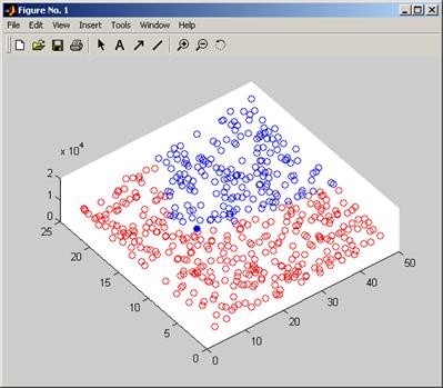
Figure 19 Plot produced by optimisationTrace
See also
view, mesh, griddata
Copyright © 2007, The Geodise Project, University of Southampton